Wooly worms
A. Degrees of freedom are 6.
C. Chi was 79.23
D.No the chi square shows that it was not chance but something caused certain worms to be picked off.
E.The worms that blended in with their environments like the pit-mans in the grass had positive selection pressure but the fire lashes in the grass stood out receiving negative pressure.
F.The results show that the worms that are not able to hide will get picked off by the birds and allow the other species to thrive.
G.The characteristics of the bird will dictate which worms the bird will be able to hunt and eat. The reason being is that certain traits in the bird will allow it to find certain worms better than others.
H. In ten years I believe that the worms that learned to take advantage of their coloration would be able to thrive. Such as the pitmans and boogies in the grass.
In the end our results were surprisingly accurate in some ways. The percent of tagged bean were 12% and our total average was 12% even though we never actually got 12% in our recaptures. Our estimate of the amounts of beans was 508.33 beans but we actually had 498 beans. I believe that some of our error came mostly from miscounting the amount of beans per recaptured samples which led to us in the end beginning slightly off in our estimate of total beans. Another factor is of course is that we could not always get the same amount of beans per capture. For example we might get 100 beans one time but maybe only 80 or 130 the ext and since we always mix the tagged beans back we do not always get a proportional amount.
There are many challenges that arose in the tagging recapture. The first problem was getting close to one hundred beans per capture. Most of the time we either got less than a hundred or we simply when over. To an actual environmental scientist this can only be worse. Because we only had to get the “animals” from a cup but they have to get them in the wild. Imagine how hard it is to get actual animals tagged and recaptured. First off it's hard to do with large animals. Think about doing this with australian Saltwater Crocodiles or with Hippos. Another problem with the size of the animal is if it is tiny, for example tagging and capturing butterflies and beetles. Of course mistake can arise with doing the math itself. Similar to how we estimated 508 individuals but thier was actually 498. It would be terrible for scientist and those trying to conserve a species.
There are many challenges that arose in the tagging recapture. The first problem was getting close to one hundred beans per capture. Most of the time we either got less than a hundred or we simply when over. To an actual environmental scientist this can only be worse. Because we only had to get the “animals” from a cup but they have to get them in the wild. Imagine how hard it is to get actual animals tagged and recaptured. First off it's hard to do with large animals. Think about doing this with australian Saltwater Crocodiles or with Hippos. Another problem with the size of the animal is if it is tiny, for example tagging and capturing butterflies and beetles. Of course mistake can arise with doing the math itself. Similar to how we estimated 508 individuals but thier was actually 498. It would be terrible for scientist and those trying to conserve a species.
1.The more diverse parking to was the students and I believe this is so because their is simply more students than there is so there is a bigger chance for the students to be more diverse.
2.The most abundant species is white cars this might be because white cars are the most produced/born species of car.
3.The student lot had a higher diversity index.
4.I believe the index would be larger in the mall parking lot because in an increase in the amount of cars and the diversity of people who drive them.
5.I believe the index will be high because an average dealership has to supply a range of vehicles and colors in order to stay in business.
Click to set custom HTML
Population Pyramids
Turlock's population seems stable. I think this is happening because birth and death rates are stable and the town is reciving as many people that are leaving.
The population in Hollister seems to be growing rapidly due to an influx of immigration.
The population of Hollister Missouri seems to be stable or slowly increasing.
The population of Hollister North Carolina seems to be unstable because of how small the amount of middle aged people there are.
Considering the small size of Ryan Town the population can be considered stable.
The population of Lexington (besides looking like a sword) is stagnate the surge of teenagers in due to the fact that Lexington is a college town.
The situation in Cut and Shoot , Texas is pretty cut and dry ; their population is rapidly declining.
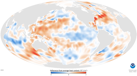
|
|
Something interesting that I noticed was the increase in tepmpature in the ice caps.
|
|
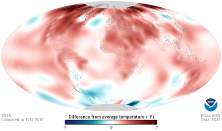
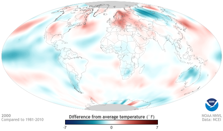
The obviously interesting difference between the two pictures is the massive difference in temperature in between 2016(left) and 2000 (right).
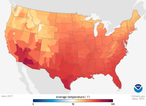
The interesting part of this is how the northwestern corner of Wyoming is fine.
